In this article, we will explore how DuckDB organizes its table structures. We’ll focus solely on the table structures while disregarding any irrelevant details.

Background Information

Block Types

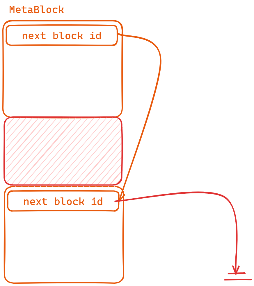
DuckDB stands out from other databases by storing all of its data within a single file. To manage this data effectively, DuckDB utilizes two types of blocks: MetaBlocks and DataBlocks.

1. A DataBlock represents an individual unit of stored information.

2. On the other hand, a MetaBlock functions as a collection of blocks with its first 8 bytes indicating the value of ‘next_block_id’. By employing such block lists when necessary due to excessive content volume.

Field Reader

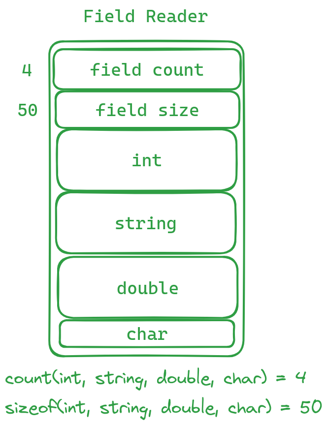
In certain cases, when retrieving data from a Block, we employ a technique called “Field Reader” for reading purposes. This “Field Reader” is independent of the table’s fields and serves as an initial step before accessing specific data by first extracting information about two key parameters: max_field_count and total_size.

1. max_field_count: Indicates the number of fields that will be retrieved afterwards.
2. total_size: Represents the overall size (in bytes) of the subsequent data retrieval process.

Segment Tree

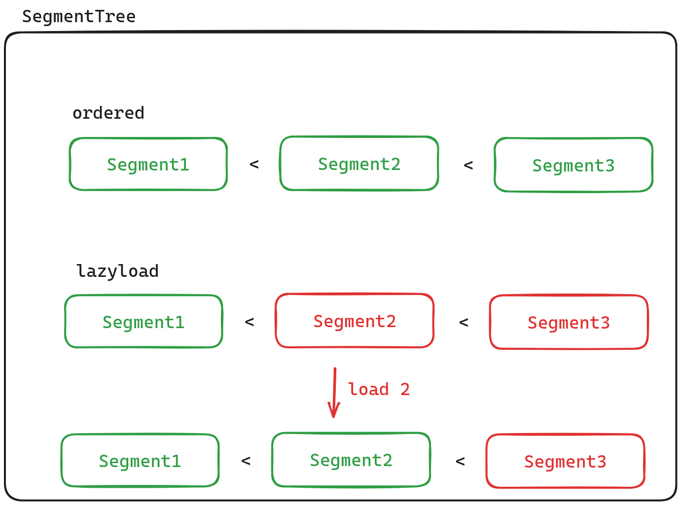
The concept of Segment refers to a block of data, and we use a data structure called segment tree (or “SegementTree”) for managing these segments. Despite its name, a segment tree internally utilizes vectors for storing segments rather than trees. Moreover, binary search is employed for locating specific segments within this structure; thus, it assumes that segments are stored in an ordered manner. One notable characteristic of segment trees is their support for lazy loading: instead of reading all segments into memory at once, they retrieve individual segments from disk on-demand.

文件结构

In this section, we will begin by introducing the file structure of DuckDB.

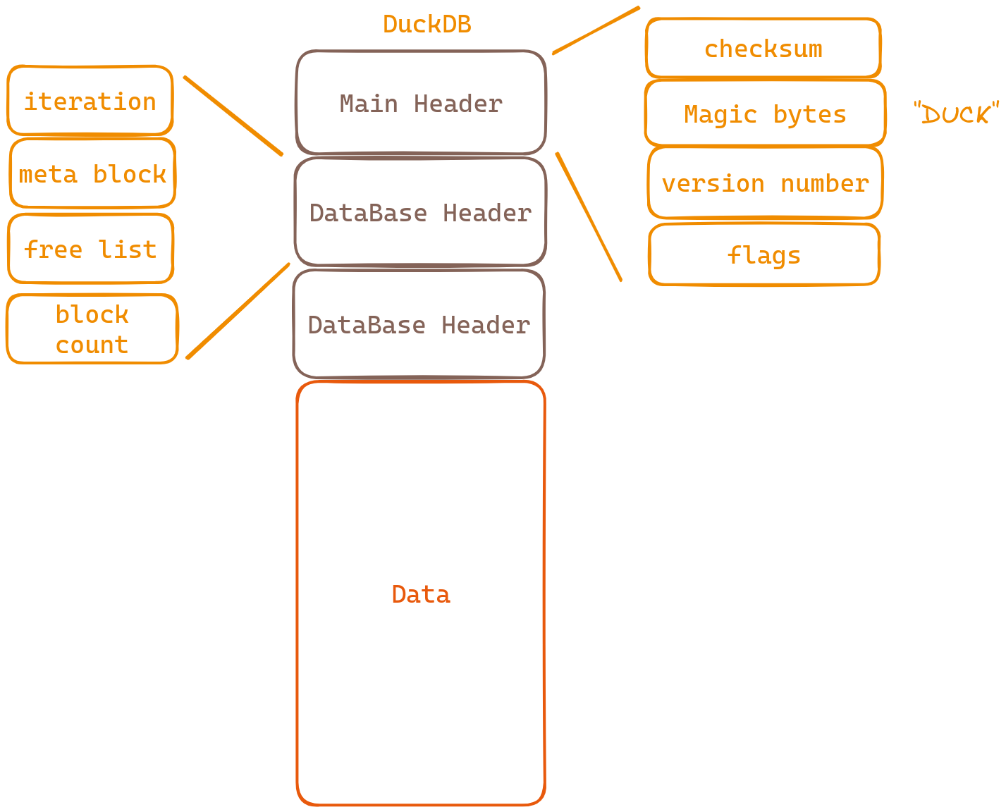
Looking at the diagram, we notice that DuckDB has three headers - but don’t worry! These headers won’t confuse us when it comes to understanding how tables are stored; they’re just some extra information we’ll briefly cover.

Let’s start with the MainHeader:

1. Checksum: A handy way to verify data integrity.
2. Magic bytes: These special bytes confirm that this file belongs to duckDB.
3. Version numbers: Keep track of software versions for compatibility purposes.
4. Flags: Indicate if you have permission to read or write on this database.

Now let’s move on to DataBaseHeader:

1. Iteration: How many times things have been iterated over (processed repeatedly).
2. Meta block: The unique identifier for the first data block in storage.
3. Free list: Blocks ready for reuse, saving space and resources.
4. Block count: The total number of blocks in the database.

Now, let’s take a look at how the actual data is stored. It consists of a schema count and ${schema_count} individual schemas. In DuckDB, think of a schema as a database.

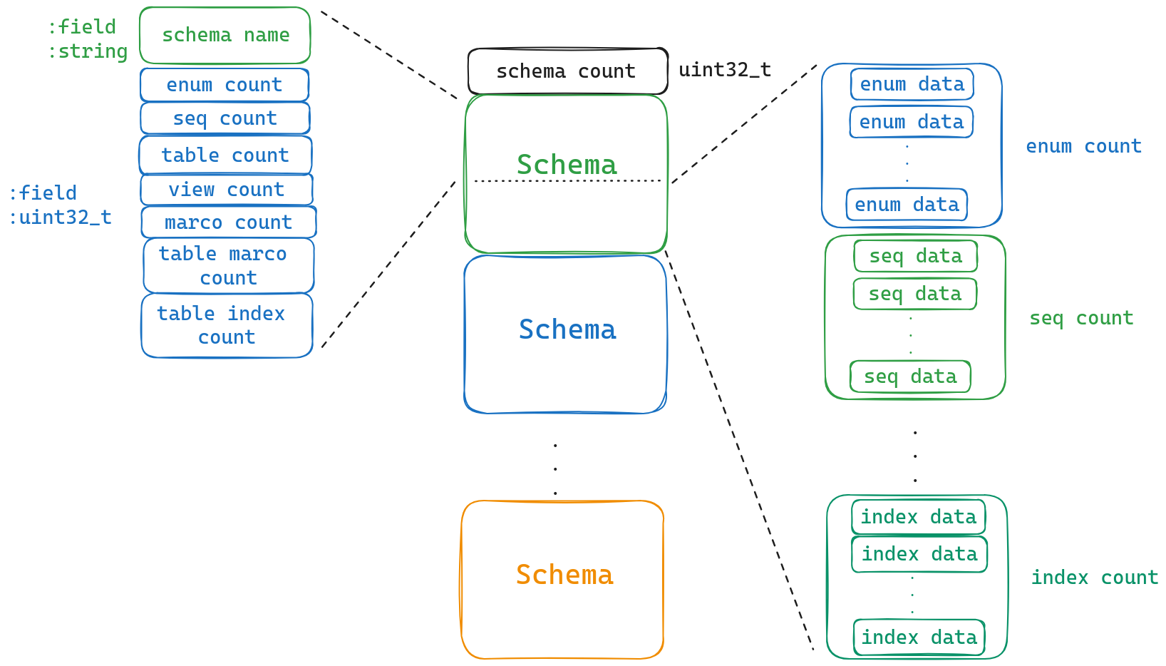
Let’s take a closer look at how schemas are stored in DuckDB databases. The first piece of information is the schema’s name, followed by a count of each type it contains. Now let’s briefly go over these different types together! For more detailed definitions, feel free to visit their official website.

1. enum
2. sequence
3. view
4. macro
5. indexes

Now, let’s shift our attention specifically to tables and explore their structures further!

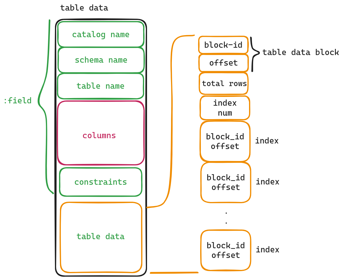
From the diagram, we can observe that the first three item in the table are labeled as catalog name,schema name and table name. By using these three items, we can identify to which file (catalog), database (schema), and specific table this particular one belongs. The field named “constraints” provides information about certain restrictions imposed on this table, such as Not Null or Unique properties. However, for now, let’s not dive too deep into this aspect; instead, let’s shift our attention towards exploring what lies within both the ‘Columns’ section and ‘table data’ field.

Columns

Within this section resides a collection of definitions for each individual column found within a given table.

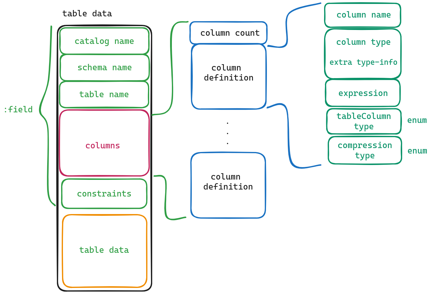
We can observe that in our dataset, the first attribute called column count which represents how many columns exist in total within our dataset file; following this attribute are individual definitions for each specific column present within our dataset file.

Now let’s delve into what each attribute signifies:

1. column name - Field name
2. column type - Field type
3. expression - Expression, some fields are generated through expressions.
4. table Column type - This is different from the column type, it does not represent the field type, but only has two values: STANDARD and GENERATED. (Actually, I’m not quite sure about the meaning of this field, it probably indicates whether this field is generated or not)
5. compression type - Indicates the compression method used for this field.

Once we have obtained information regarding the types and characteristics of each column, we gain comprehensive knowledge about the overall structure and organization of our dataset. The remaining components consist of actual data entries and index-related information, which can be accessed through the table data field.

table data

Since indexes and table data are usually large in size, we don’t store them directly here. Instead, we store pointers (block-id, offset) that point to their actual locations.

Let’s explain each field using this diagram:

1. table data block: Pointer to the actual table data.
2. total rows: The number of rows in this table.
3. index num: The total number of indexes in this table.
4. index: Pointer to the index.

Now let’s examine how table data block stores its actual structured information.

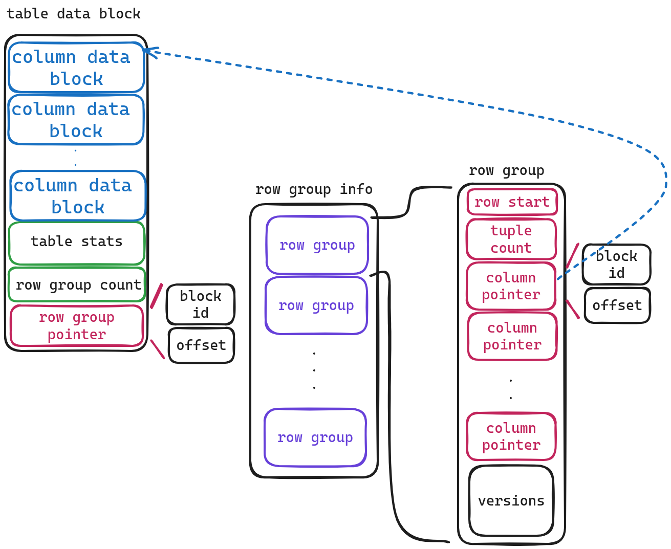
The initial storage contains metadata about a series of column data (the structure of the column data block will be explained later). The last two fields are easy to understand. The first one stores statistical information about the table, and the other one stores the number of ‘row groups’. Now, let’s address two questions: what is a ‘row group’, and why is the storage format different from before, which was <data-count, data, data,...data>, but now only stores a ‘row group pointer’? What happens if there are more than 1 ‘row group’?

row group

We all know that OLAP generally uses columnar storage while OLTP uses row-based storage. Although columnar storage is superior in terms of reading and computation, when it comes to frequent insertions, deletions or updates, row-based storage outperforms columnar storage. Therefore, DuckDB has come up with a compromise here by grouping tuples and storing them in columns within each group. Currently, every 122880 tuples form one group.

Why only one row group pointer?

Because row groups are always stored sequentially according to their line numbers and they store blocks as meta blocks. Hence they can be managed through a SegmentTree for lazy loading subsequent row groups. When needed, they can be read directly from behind. That’s why we only need to store the block-id of the first block here.

Now let’s take a look at the storage structure of row groups.

1. Row start: The starting line number of this row group.
2. Tuple count: The number of rows in this row group.
3. Column pointers: Since columns are stored within each row group vertically (column-wise), this pointer points to the actual storage address for each column.
4. Versions: I haven’t looked into this field too closely; it should be related to MVCC.

Let’s continue with the storage structure of column data blocks.

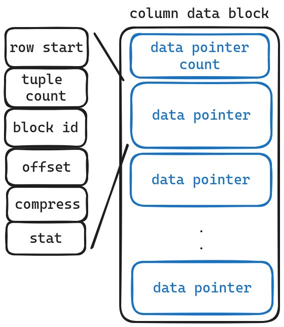
To our surprise, we discovered that this isn’t actually where the data itself is stored; it still holds pointers instead! But why? Well, it turns out that the real column data resides in what’s called “pure blocks.” Unlike their counterparts known as “meta blocks,” these pure blocks don’t have a convenient way to keep track of all their contents using a simple list structure like before.

As usual, let’s explain the meanings of each field:

1. row start: The starting row number of this data.
2. tuple count: The total number of rows stored.
3. block id: The block ID where the actual data resides.
4. offset: The offset within the block ID where the actual data resides.
5. compress: The compression method used for the data.
6. stat: Statistical information about this portion of data.

Now, we’ve finally arrived at the very heart of it all—the block housing our precious columnar data! However, please note that its storage format can vary depending on which compression technique was employed during processing. I’ll briefly introduce a few common types here, but if you’re curious about others, feel free to explore them further on your own!

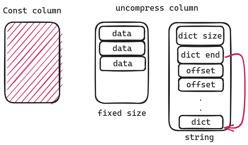
Const Column

In a const column, every single value is identical. This means we don’t need to store any actual data at all. Instead, we can simply retrieve the minimum value from the statistical information.

uncompress column

When it comes to uncompressing columns in a dataset, it means that there is no compression applied to these specific columns. For data types such as uint32 or uint8, which have fixed sizes, we can easily read each value individually without any additional steps required. However, when dealing with variable-length data types like strings that do not have predetermined lengths, a different approach called Dictionary Compression is used

For strings, the first two fields give us the position of the dictionary:

1. dict_start = dict_end - dict_size
2. dict_end = dict_end
3. dict_size = dict_size

Here, we can consider the dictionary as a string pool and offsets as corresponding starting positions, where offsets[i] - offsets[i-1] represents the length. This might sound abstract, so let’s take an example.

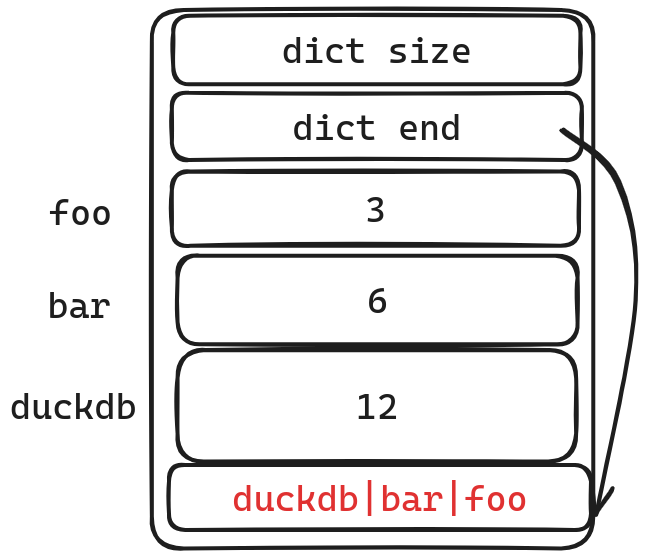
In this example, we have three strings: foo, bar, and duckdb.

We store these three strings in reverse order in a dictionary. The offset is relative to the “dict end”. This allows us to locate the starting address of the corresponding string.

1. foo
   head = dict - offset = dict - 3

   length = 3 - 0 = 3

2. bar
   head = dict - offset = dict - 6

   length = 6 - 3 = 3

3. foo
   head = dict - offset = dict - 12

   length = 12 - 6=6

Now, let’s address a potential issue: what if a string exceeds the maximum allowed length? In such cases, we utilize negative offsets to indicate that these strings are longer than usual. To access them, we store their (block id, offset) pairs in our dictionary and retrieve them from another block where they are stored.

RLE column and bitpacking

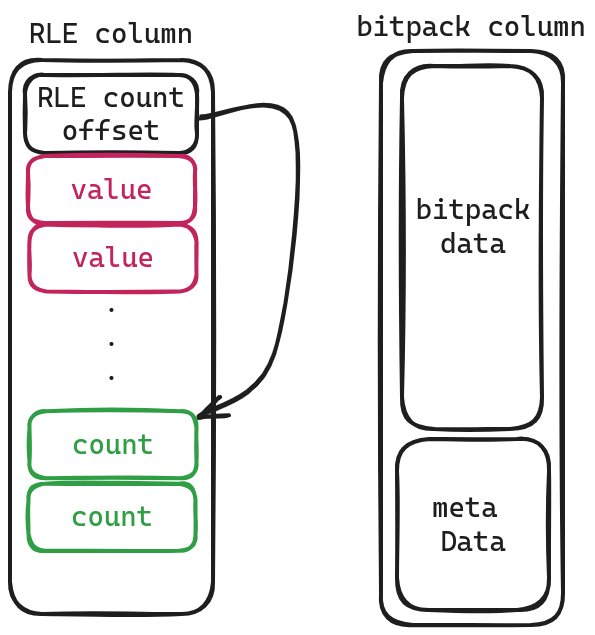
RLE column is relatively simple, with the values stored in the front and the number of occurrences of each value stored in the back. They are separated by RLE count offset.

As for bitpack columns, I’ll let curious readers delve into that topic themselves.

Dictionary column

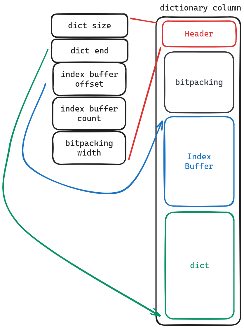
If you grasp how strings are stored in “uncompress column,” understanding “Dictionary column” becomes much easier as well. In this case, the term ‘dict’ retains its original meaning while ‘index Buffer’ refers to what was previously mentioned as ‘offsets’ and ‘bitpacking.’ It represents which position within the index Buffer corresponds to each row’s value. By using dict.get(indexBuffer[bitpacking[i]]), we can retrieve the stored value.

One important optimization technique employed here involves decompressing the dict during actual scanning. However, if it turns out that all data needs to be scanned, only decompressing bitpacking would suffice.

Last

In this article, we explored how tables are stored in DuckDB. Unlike other databases, DuckDB takes a unique approach by utilizing just one file to store all of its data (although I’m unsure whether this is advantageous or not). Designed as a single-machine database without distributed capabilities in mind, it aims to optimize performance through techniques such as lazy loading with row groups. Additionally, column data can be compressed using various formats for efficient storage.