Vector search, like text search, isn’t just about returning accurate results at low latency — it often has to do so under certain constraints as well, that is, with filtering.

For text search this isn’t a problem: an inverted index is essentially a “hash table + linked list” structure, so we just drop the documents that don’t match the condition as we walk the linked list. Vector search, however, can’t handle this nearly as gracefully, as we’ll unpack below.

Note: by “vector search algorithm” here we specifically mean graph-based algorithms like HNSW.

Why is filtering hard for vector search?

Post Filter

The most intuitive idea for filtering is to compute the results first, then throw away whatever doesn’t meet the requirement. It’s a valid approach, but it runs into a structural conflict with vector search: there’s no such thing as a vector that “doesn’t meet the requirement” — all we measure is the relative distance between vectors. So for vector search, everything is about TopK (the K nearest vectors by distance). If we compute the TopK vectors first and then filter them by the condition, the final result count shrinks — and can even drop to zero (the user wants the 100 nearest vectors but only gets 30 back, or even 0 — not because there are no matching vectors, but because they were filtered out).

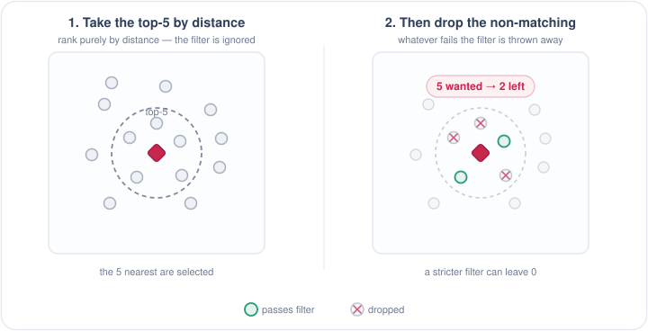
Post-filter ranks by distance first, then drops whatever fails the filter — the result can be far smaller than k, and a strict filter can leave nothing at all.

At this point, a natural next thought is: in that case, just search for more up front — if the user wants 100, search for 1000 first, so that after filtering we can still gather 100 to return. But this leads to two problems:

1. Over-fetching hurts performance — search not only has to recall the correct documents, it also has to finish within a tight latency budget.
2. You can’t guarantee that over-fetching will leave enough results to return: if the filter is strict, even searching for 10× as many may still come back empty.

Pre Filter

Since filtering after searching brings so many problems, can we do the reverse — first find all the vectors that satisfy the filter condition, then pick the nearest TopK from among them?

This approach can solve the problem too, but once we’ve pulled out all the matching vectors, we’ve lost HNSW’s graph structure and can only compute distances to these vectors one by one. If most points satisfy the filter, this is no different from a brute-force search over the entire dataset, and the latency is unacceptable.

That said, Pre Filter isn’t worthless — how expensive it is depends entirely on the match rate of the filter. When the condition is very strict and only a few vectors match, the candidate set itself is small, and brute-forcing it directly is actually the fastest; only when the match rate is high and most vectors pass does it degrade into a full-database scan. In other words, Post Filter and Pre Filter are each only good within a certain band of match rates — neither approach can cover every scenario.

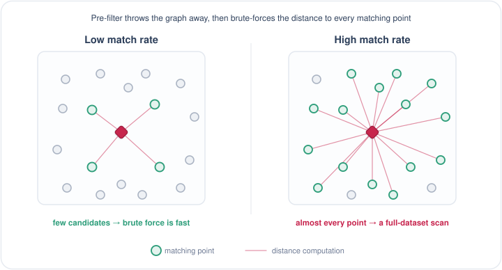
Pre-filter discards the graph and scans the matching points one by one: fast when few match, but it degrades into a near-full-dataset scan once most points pass.

Today’s mainstream filtering algorithms

Since neither of these naive ideas solves the problem well, let’s look at the mainstream filtering algorithms used on HNSW today.

Note: from here on we’ll dive straight into the specific filtering algorithms, assuming you already have some understanding of how HNSW search itself works.

result-gate filtering

result-gate filtering has no official name; it’s the default approach used by hnswlib. To explain it clearly, we first need to recall how HNSW searches within a single layer.

First, plain HNSW search. It maintains two sets:

• candidate-set (C): the points still to be explored, which decide “which direction to walk next in the graph”;
• result-set (W): the nearest points found so far, which will ultimately be returned to the user.

The search repeatedly pops from C the point c nearest to the query and examines each of its neighbors e: as long as e is closer than the farthest point in W (or W hasn’t yet collected ef points), e is pushed into both C and W.

SEARCH-LAYER(q, ep, ef):
  C ← {ep}                # candidate set, ordered by distance to q (nearest first)
  W ← {ep}                # result set, keeps the ef nearest found so far
  visited ← {ep}
  while C is not empty:
    c ← extract nearest point to q from C
    if dist(c, q) > dist(furthest in W, q):
      break                                # cannot improve anymore, stop
    for e in neighbors(c):
      if e in visited: continue
      visited.add(e)
      if dist(e, q) < dist(furthest in W, q) or |W| < ef:
        C.add(e)                           # admit to candidate set
        W.add(e)                           # admit to result set
        if |W| > ef: remove furthest from W
  return W

In the original HNSW algorithm, whether a point can enter C and whether it can enter W are actually judged by the same condition: whether it’s close enough to the query.

What result-gate filtering does is split that single decision — “can this point enter C” versus “can it enter W” — into two separate conditions.

We don’t change the condition for entering the candidate-set, so the search’s routing path is unchanged — it still follows the original route. The graph’s connectivity is also the same as without filtering, so filtering doesn’t degrade the quality of the routing path. We only add one extra check when entering the result-set: besides satisfying the distance requirement of the path, a point must also satisfy the filter condition. In code, that’s just one extra line:

    for e in neighbors(c):
      if e in visited: continue
      visited.add(e)
      if dist(e, q) < dist(furthest in W, q) or |W| < ef:
        C.add(e)                           # admit to candidate set: unchanged
        if filter(e):                      # ★ the only change
          W.add(e)                         # admit to result set only if filter passes
          if |W| > ef: remove furthest from W

So what does this filtering algorithm actually achieve? First, it still walks the graph, and the walk follows the same path as the no-filter search, which means it still rapidly converges toward the TopK results — speed is guaranteed. As for the result count, because HNSW keeps searching as long as W hasn’t collected ef points, the search keeps probing outward on its own, until it really has found ef matching points or the entire graph has been searched. So we won’t run into the empty-result situation that Post Filter has.

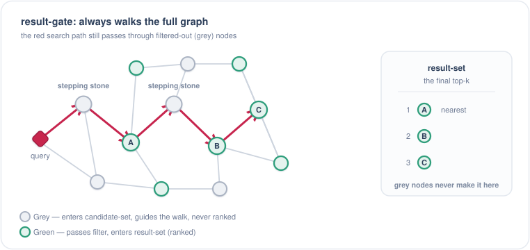
The search path still walks through the grey nodes — they enter the candidate-set and guide the walk — but only matching green nodes make it into the result-set. Guides the walk, never ranked.

ACORN

ACORN comes from this paper, which proposes two algorithms: ACORN-γ and ACORN-1. Here we only cover ACORN-1 — because ACORN-γ has a high graph-construction cost and requires rebuilding the index, almost nobody uses it in practice; ACORN-1, on the other hand, can run directly on an existing HNSW index, with very low implementation cost.

The idea behind ACORN-1 is actually quite simple. Since what we’re after is the TopK that satisfy the filter, we might as well, during the search, only put matching points into the candidate-set and only compute distances for those points, discarding non-matching points outright. This is exactly the opposite of result-gate from the previous section — in result-gate, non-matching points also enter the candidate-set and take part in the computation. The benefit is that it saves a large amount of distance computation.

But this has a side effect: if the filter is strict and the matching points are sparse, the graph’s connectivity can’t be preserved. In the HNSW graph every point was originally connected, but once we delete all the non-matching points, the graph gets split into separate subgraphs — quite possibly two matching points were connected only through a non-matching point, and deleting it breaks the link. The result is that we may just spin around in a small patch of the graph, unable to get out.

To solve this, ACORN uses Neighbor Expansion to repair connectivity. When we arrive at a point and inspect its neighbors: if a neighbor satisfies the filter, we compute its distance and add it to the candidate-set as usual; but if the neighbor doesn’t satisfy the filter, instead of discarding it outright, we follow it one more hop and pull out its neighbors to inspect too. In other words, a non-matching point is treated as a “bridge” — we cross over it to see whether there are other matching points beyond. This is where “two hops” comes from — the first hop lands on the non-matching neighbor, the second hop reaches the matching point behind it, and two points that the filter had disconnected are reconnected.

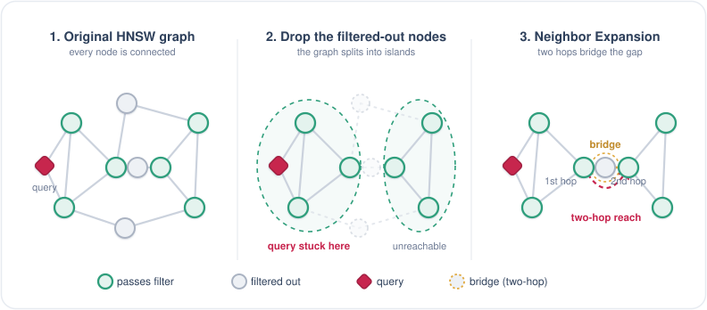
① the full graph is connected → ② keeping only the matching nodes shatters it into islands and traps the query → ③ Neighbor Expansion bridges the grey nodes in two hops to reconnect the far side.

So ACORN-1 saves a large amount of distance computation by “only computing matching points,” while patching connectivity back with two-hop Neighbor Expansion — all in the hope of completing the filtered search quickly.

Although ACORN’s idea is appealing, getting it to actually land in production takes some engineering work — the best example being Lucene’s implementation. On top of ACORN, Lucene makes three main changes:

1. Lazy expansion: the original ACORN does two hops unconditionally — regardless of whether there are enough matching neighbors, it always expands the non-matching ones. Lucene argues this is unnecessary and switches to on-demand expansion: it first computes distances for the matching neighbors, and if there are already enough qualified neighbors in this hop, no further expansion is needed; only when the qualified neighbors are insufficient does it do the second hop on the non-matching ones. This preserves connectivity while saving a lot of unnecessary expansion.
2. Multi-hop: if the graph’s connectivity turns out to be especially poor and two hops aren’t enough, it keeps going to three hops, four hops, and so on, until it has gathered enough qualified points.
3. Explore budget: it sets an upper bound on the exploration volume and adjusts it dynamically based on selectivity, to avoid exploring endlessly in extreme cases.

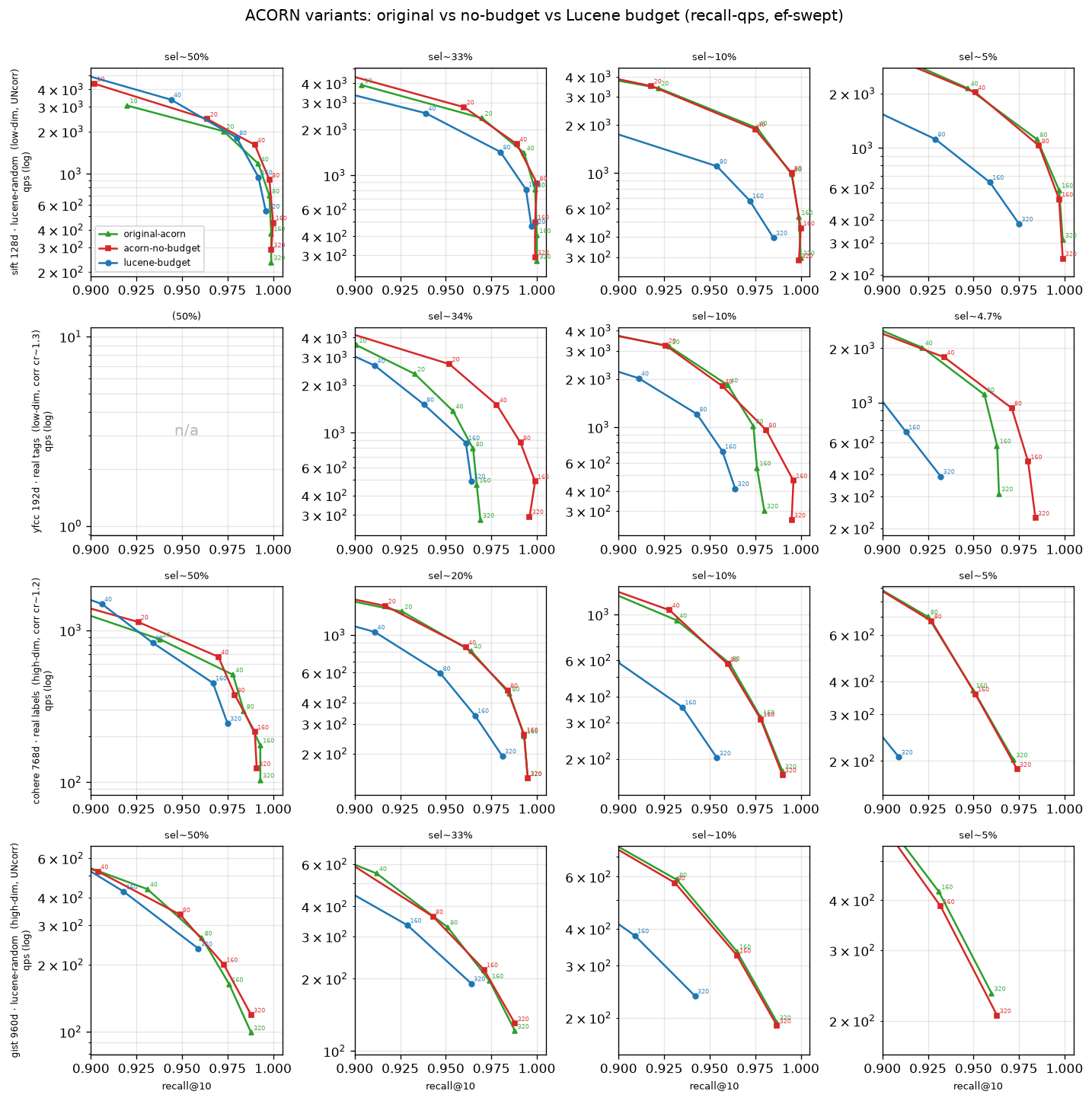
In my own experiments, the first two changes both give small improvements over the original ACORN, but the third one — the explore budget — is actually worse. I think the reason is that once you set an upper bound, the search latency does become more predictable and there’s no tail-latency blowup in extreme cases; but the cost is worse routing quality — although the budget caps the exploration at each step, it makes the search more likely to wander off course, so to reach the same recall it ends up visiting many more points across the graph, and the average latency goes up.

The figure below puts three qps-recall curves side by side: ACORN with the explore budget, without it, and the original paper version. As you can see, the version without it is actually the best. So in the next section’s comparison of filtering algorithms, we use this no-explore-budget version of ACORN and compare it against result-gate.

Comparing the filtering algorithms

Before the formal comparison, a word on the datasets used and their filter conditions:

• SIFT1M / GIST1M: the filtered points are chosen at random (a random filter);
• YFCC1M: uses the dataset’s own real image tags as the filter;
• Cohere1M: uses the dataset’s own real scalar labels as the filter.

Let’s first look at the comparison between ACORN and result-gate on these four datasets:

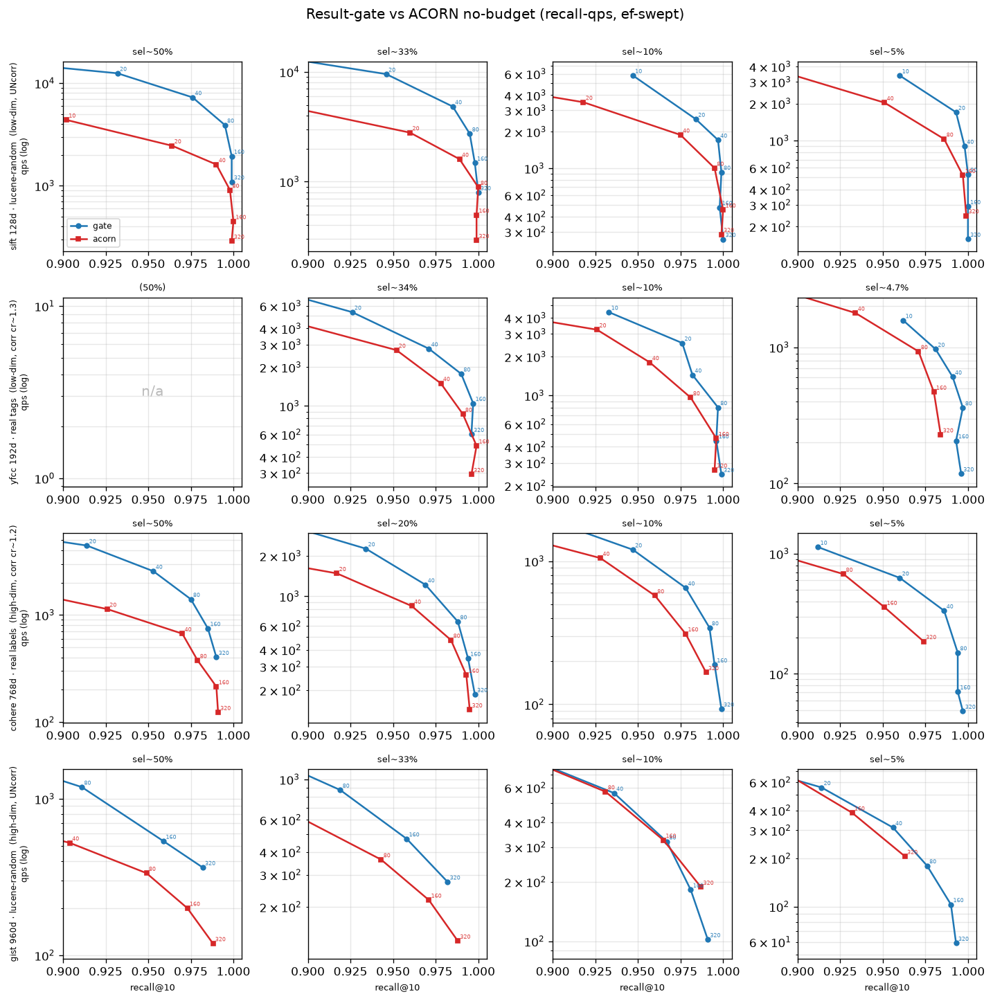
From the figure, at the same recall, ACORN loses to result-gate in most cases. So why is that? ACORN went to all this trouble precisely to compute fewer distances — why is its performance still no match for result-gate? There are two reasons.

Root cause one: HNSW’s bottleneck is memory access, not distance computation.

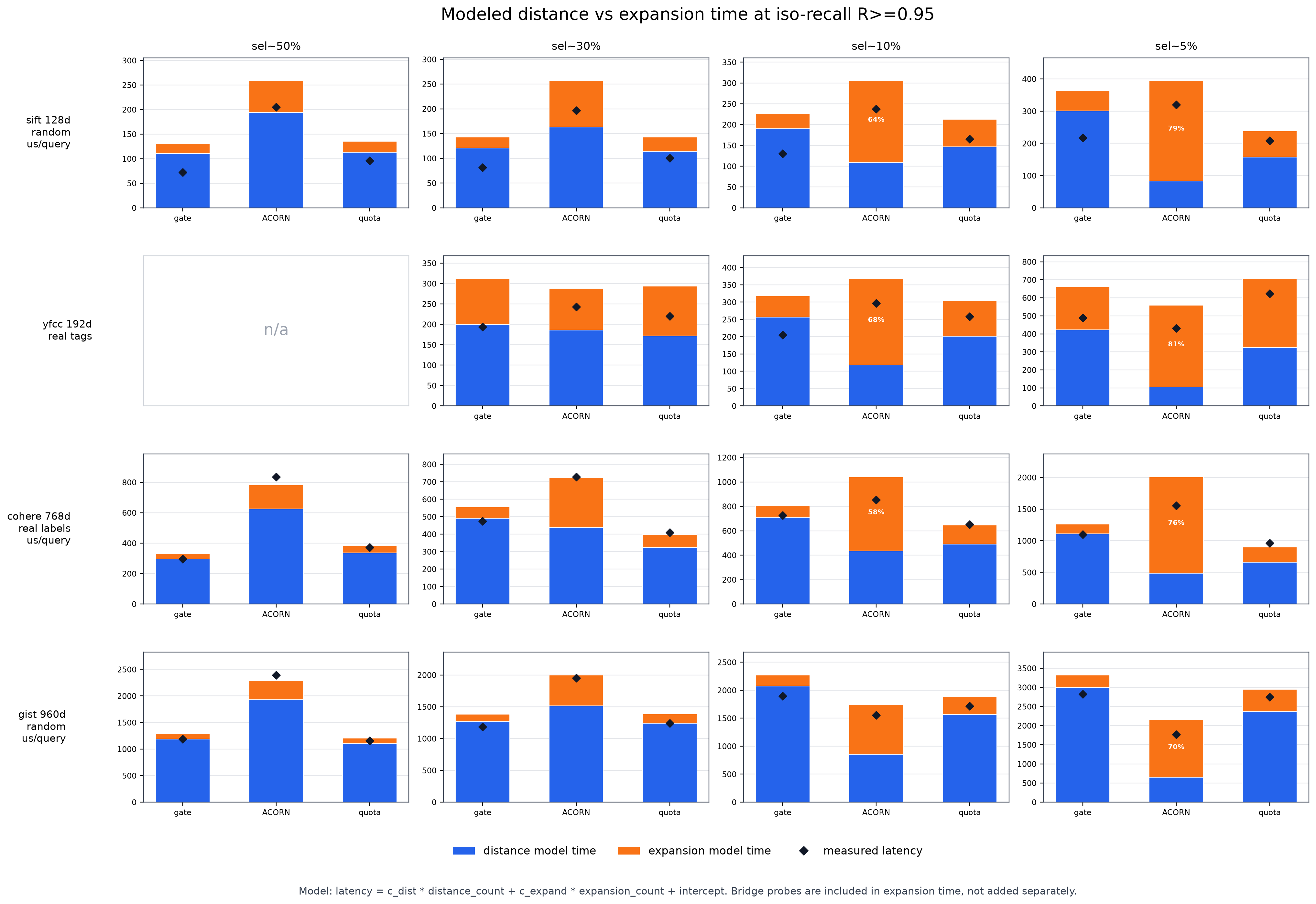
If we look at the hot functions during HNSW search, we’ll find that the vast majority of time goes to distance computation. But that doesn’t mean the time is really spent on the CPU computing distances — in fact, most of it is still spent on memory access (fetching the vectors out of memory). For low-dimensional datasets like SIFT and YFCC, with SIMD + prefetch a single distance computation touches very little memory. So the little gain ACORN gets from computing fewer distances doesn’t outweigh the overhead of its node expansion (more memory accesses, more pointer hops). The figure below makes it clear: the distance-computation time does drop sharply, but the expansion time rises even more.

Root cause two: ACORN saves on distance computation, but the routing quality drops along with it.

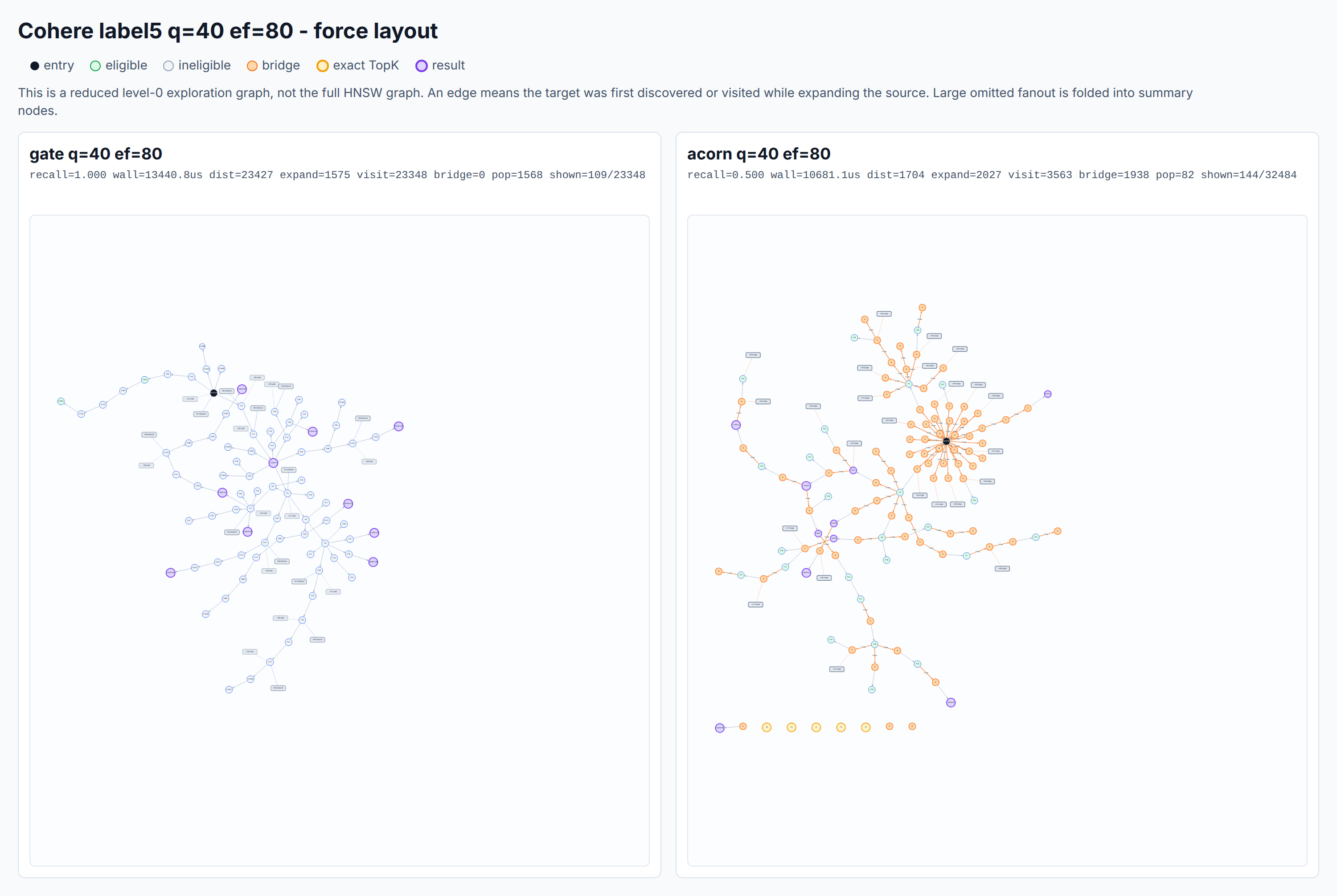
On low-dimensional data, distances are cheap and ACORN can’t gain anything — that’s understandable. But why, even on high-dimensional data, does ACORN still fail to beat result-gate? The problem is routing. ACORN only walks among the “points that satisfy the filter,” which is like navigating on a sparse graph that’s been hollowed out and then barely patched back together with two hops; result-gate, meanwhile, always walks on the original complete graph (where non-matching points can still help guide the way). So ACORN’s routing quality is inherently worse than result-gate’s, and to reach the same recall it has to set ef larger — and once ef grows, latency naturally goes up. The figure below shows the difference between the two during the search.

So to sum up, for ACORN to beat result-gate, several conditions must hold at the same time:

1. The vector dimensionality is high enough.
2. The filter is strict enough (low match rate, only a few points pass).
3. The filter must be correlated with the vector distribution — that is, the points satisfying the filter must also lie close to one another in vector space.

The first two are easy to understand; let me explain the third a bit. For example: if your vectors come from music embeddings, then the filter had better be music-related too — because ACORN’s whole approach implicitly assumes that the points satisfying the filter are themselves clustered together. If the filter is completely unrelated to the vectors, the matching points are scattered across every corner of the graph, ACORN’s two hops can hardly string them together, and the results naturally won’t be good.

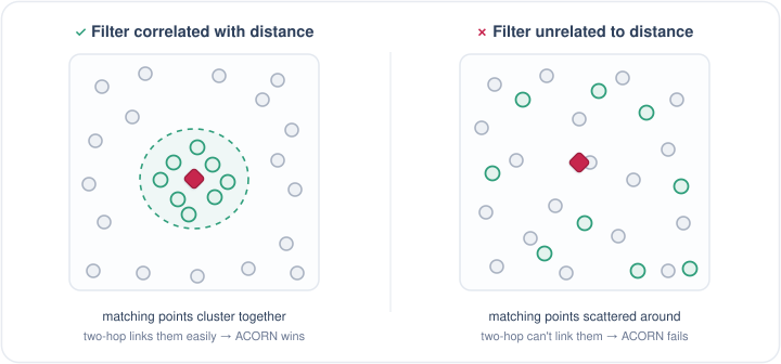
Left: the matching points cluster, so two-hop links them and ACORN wins. Right: the matching points are scattered, two-hop can’t reach them, and ACORN fails.

One More Thing

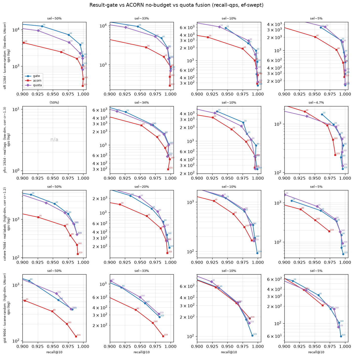
There’s a powerful idea in computer science called “fusion” — merging two methods into a single, better one. Following this line of thought, we can consider an algorithm that combines result-gate and ACORN (although, in practice, it didn’t manage to consistently beat either one).

The idea goes like this: ACORN’s routing is poor because it only puts matching points into the candidate-set. So we can strike a compromise — when iterating over a point’s neighbors, first compute only the matching points; if there are enough, carry on the ACORN way; if there aren’t, fall back to result-gate’s approach and visit the non-matching points directly, borrowing them to restore routing quality.

That leaves just one question: exactly how many matching points count as “enough,” so that we don’t have to touch the non-matching ones?

We can use a bit of probability here to estimate this threshold. The intuition is: as long as there are enough direction-providing points among the one-hop neighbors, there’s a high probability we’ve already covered the top p% of nearest neighbors, and at that point we don’t need to touch the non-matching ones. I’ve put the full derivation in the appendix at the end; here I’ll just give the conclusion — we use an empirical threshold that adapts to the match rate $s$: the looser the filter, the more matching neighbors there already are; the stricter the filter, the more result-gate-style routing capability it automatically adds back.

The comparison of the three algorithms is below.

Conclusion

After all this, the conclusion really comes down to one thing: there is no silver bullet. No single algorithm consistently wins across every scenario; the only thing you can do is pick the one best suited to your own workload.

And if you have no idea what your workload even looks like, just go with result-gate without overthinking it: it’s the simplest to implement, and it still works very well.

Appendix: deriving the threshold for the fused algorithm

Suppose each point at level 0 has at most $M_0$ neighbors, and the filter’s match rate is $s$. Then among a point’s one-hop neighbors, we expect $M_0 \cdot s$ of them to satisfy the filter. These would be distance-computed by ACORN anyway; if we want at least $K$ direction-providing neighbors at each step, we only need to top up from the non-matching neighbors by:

points.

Next we need to estimate: by topping up $r$ points, do we have a high probability of hitting a “good enough routing direction”? If we treat the top $p$ fraction of neighbors closest to the query as good directions, then drawing $r$ out of $M_0$ neighbors, the probability of hitting at least one good direction is:

Conversely, if we want the hit probability to be at least $\alpha$, then:

For example, taking $p=1/4$ and $\alpha=95\%$, at $M_0=32$ topping up about 9 to 11 neighbors gives a high probability of hitting a top-25% nearest-neighbor direction.

In the end, though, we didn’t plug this theoretical value in directly, because it’s a bit conservative. In practice, a better empirical threshold turned out to be:

That is: first account for the expected number of matching neighbors, then add a small constant term independent of $s$ as a “baseline sample” of routing directions. When the filter is loose, there are already plenty of matching neighbors; when the filter is strict, this extra term adds back a bit of result-gate-style routing capability.